Compute Eigenvalues using PyAnsys Math and SciPy

This example shows how to perform these tasks:

• Extract the stiffness and mass matrices from an MAPDL model.

• Use PyAnsys Math to compute the first eigenvalues.

• Get these matrices using SciPy to obtain the same solutions using Python resources.

• See if PyAnsys Math is more accurate and faster than SciPy.

Perform required imports and start PyAnsys Math

Perform required imports.

import math
import time

from ansys.mapdl.core.examples import examples
import matplotlib.pylab as plt
import numpy as np
import scipy
from scipy.sparse.linalg import eigsh

import ansys.math.core.math as pymath

# Start PyAnsys Math as a service.
mm = pymath.AnsMath()

Load the input file

Load the input file using MAPDL.

print(mm._mapdl.input(examples.wing_model))

/INPUT FILE= wing.dat  LINE=       0

*** WARNING ***                         CP =       0.966   TIME= 15:01:41
The /BATCH command must be the first line of input.  The /BATCH command
is ignored.

*** MAPDL - ENGINEERING ANALYSIS SYSTEM  RELEASE                  24.1     ***
Ansys Mechanical Enterprise Academic Student
01055371  VERSION=LINUX x64     15:01:41  APR 22, 2024 CP=      0.967





         ***** MAPDL ANALYSIS DEFINITION (PREP7) *****

*** WARNING ***                         CP =       0.967   TIME= 15:01:41
Deactivation of element shape checking is not recommended.

*** WARNING ***                         CP =       1.004   TIME= 15:01:41
The mesh of area 1 contains PLANE42 triangles, which are much too stiff
in bending.  Use quadratic (6- or 8-node) elements if possible.

*** WARNING ***                         CP =       1.015   TIME= 15:01:41
CLEAR, SELECT, and MESH boundary condition commands are not possible
after MODMSH.


***** ROUTINE COMPLETED *****  CP =         1.019

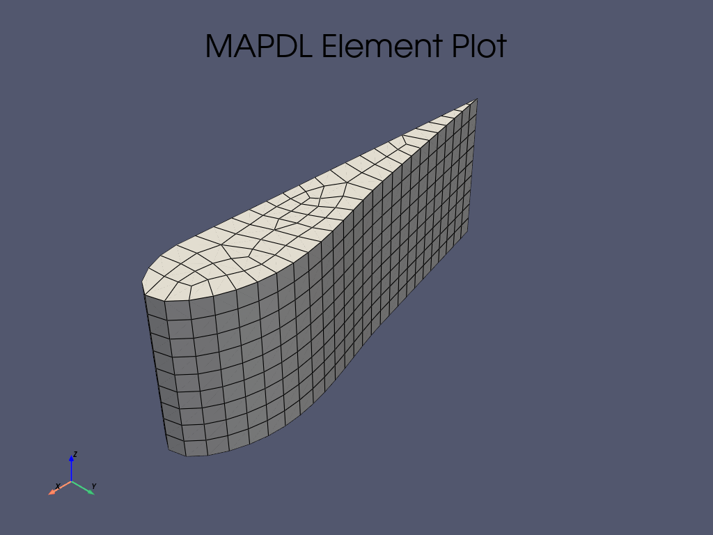
Plot and mesh

Plot and mesh using the eplot method.

mm._mapdl.eplot()

Static Scene

Interactive Scene

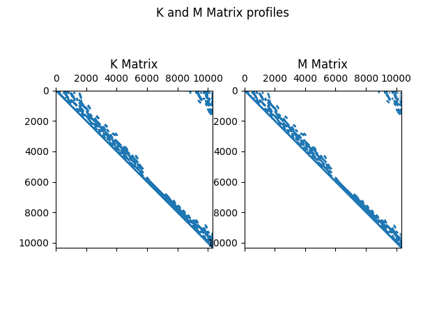
Set up modal analysis

Set up a modal analysis and form the \(K\) and \(M\) matrices. MAPDL stores these matrices in a .FULL file.

print(mm._mapdl.slashsolu())
print(mm._mapdl.antype(antype="MODAL"))
print(mm._mapdl.modopt(method="LANB", nmode="10", freqb="1."))
print(mm._mapdl.wrfull(ldstep="1"))

# store the output of the solve command
output = mm._mapdl.solve()

*****  MAPDL SOLUTION ROUTINE  *****
PERFORM A MODAL ANALYSIS
  THIS WILL BE A NEW ANALYSIS
USE SYM. BLOCK LANCZOS MODE EXTRACTION METHOD
  EXTRACT    10 MODES
  SHIFT POINT FOR EIGENVALUE CALCULATION=  1.0000
  NORMALIZE THE MODE SHAPES TO THE MASS MATRIX
STOP SOLUTION AFTER FULL FILE HAS BEEN WRITTEN
   LOADSTEP =    1 SUBSTEP =    1 EQ. ITER =    1

Read sparse matrices

Read the sparse matrices using PyAnsys Math.

mm._mapdl.finish()
mm.free()
k = mm.stiff(fname="file.full")
M = mm.mass(fname="file.full")

Solve eigenproblem

Solve the eigenproblme using PyAnsys Math.

nev = 10
A = mm.mat(k.nrow, nev)

t1 = time.time()
ev = mm.eigs(nev, k, M, phi=A, fmin=1.0)
t2 = time.time()
pymath_elapsed_time = t2 - t1
print("\nElapsed time to solve this problem : ", pymath_elapsed_time)

Elapsed time to solve this problem :  0.4790050983428955

Print eigenfrequencies and accuracy

Print the eigenfrequencies and the accuracy.

Accuracy : \(\frac{||(K-\lambda.M).\phi||_2}{||K.\phi||_2}\)

pymath_acc = np.empty(nev)

for i in range(nev):
    f = ev[i]  # Eigenfrequency (Hz)
    omega = 2 * np.pi * f  # omega = 2.pi.Frequency
    lam = omega**2  # lambda = omega^2

    phi = A[i]  # i-th eigenshape
    kphi = k.dot(phi)  # K.Phi
    mphi = M.dot(phi)  # M.Phi

    kphi_nrm = kphi.norm()  # Normalization scalar value

    mphi *= lam  # (K-\lambda.M).Phi
    kphi -= mphi

    pymath_acc[i] = kphi.norm() / kphi_nrm  # compute the residual
    print(f"[{i}] : Freq = {f:8.2f} Hz\t Residual = {pymath_acc[i]:.5}")

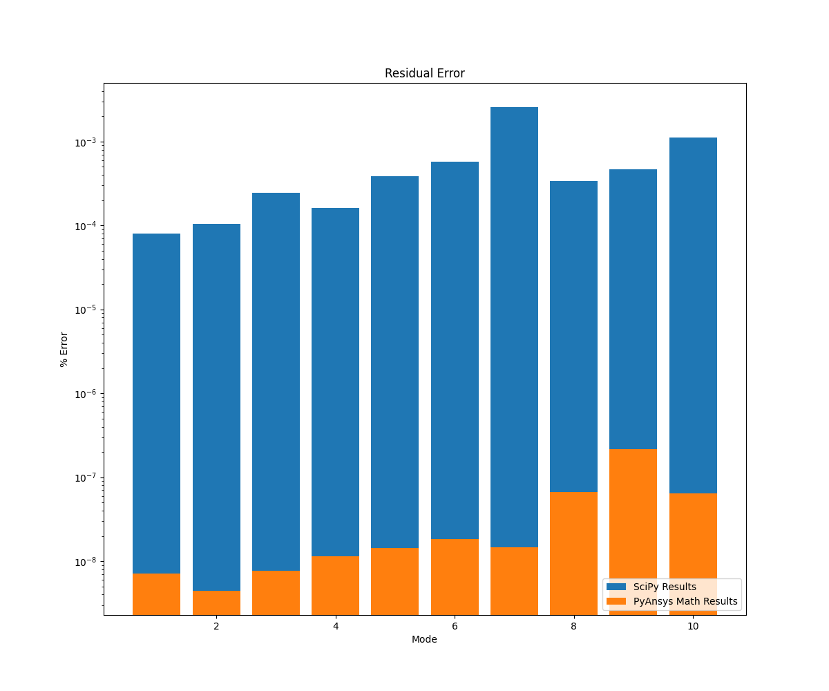
[0] : Freq =   352.39 Hz         Residual = 7.1398e-09
[1] : Freq =   385.20 Hz         Residual = 4.4352e-09
[2] : Freq =   656.78 Hz         Residual = 7.6434e-09
[3] : Freq =   764.73 Hz         Residual = 1.1473e-08
[4] : Freq =   825.49 Hz         Residual = 1.4281e-08
[5] : Freq =  1039.25 Hz         Residual = 1.8512e-08
[6] : Freq =  1143.60 Hz         Residual = 1.4537e-08
[7] : Freq =  1258.00 Hz         Residual = 6.6247e-08
[8] : Freq =  1334.23 Hz         Residual = 2.154e-07
[9] : Freq =  1352.10 Hz         Residual = 6.4539e-08

Use SciPy to solve the same eigenproblem

Get the MAPDL sparse matrices into Python memory as SciPy matrices.

pk = k.asarray()
pm = M.asarray()

# get_ipython().run_line_magic('matplotlib', 'inline')

fig, (ax1, ax2) = plt.subplots(1, 2)
fig.suptitle("K and M Matrix profiles")
ax1.spy(pk, markersize=0.01)
ax1.set_title("K Matrix")
ax2.spy(pm, markersize=0.01)
ax2.set_title("M Matrix")
plt.show(block=True)

Make the sparse matrices for SciPy unsymmetric because symmetric matrices in SciPy are memory inefficient.

\(K = K + K^T - diag(K)\)

pkd = scipy.sparse.diags(pk.diagonal())
pK = pk + pk.transpose() - pkd
pmd = scipy.sparse.diags(pm.diagonal())
pm = pm + pm.transpose() - pmd

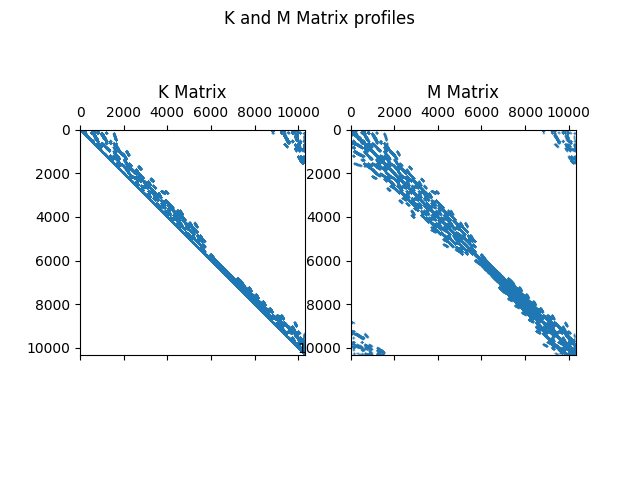
Plot the matrices.

fig, (ax1, ax2) = plt.subplots(1, 2)
fig.suptitle("K and M Matrix profiles")
ax1.spy(pk, markersize=0.01)
ax1.set_title("K Matrix")
ax2.spy(pm, markersize=0.01)
ax2.set_title("M Matrix")
plt.show(block=True)

Solve the eigenproblem.

t3 = time.time()
vals, vecs = eigsh(A=pK, M=pm, k=10, sigma=1, which="LA")
t4 = time.time()
scipy_elapsed_time = t4 - t3
print("\nElapsed time to solve this problem : ", scipy_elapsed_time)

Elapsed time to solve this problem :  2.037623405456543

Convert lambda values to frequency values: \(freq = \frac{\sqrt(\lambda)}{2.\pi}\)

freqs = np.sqrt(vals) / (2 * math.pi)

Compute the residual error for SciPy.

\(Err=\frac{||(K-\lambda.M).\phi||_2}{||K.\phi||_2}\)

scipy_acc = np.zeros(nev)

for i in range(nev):
    lam = vals[i]  # i-th eigenvalue
    phi = vecs.T[i]  # i-th eigenshape

    kphi = pk * phi.T  # K.Phi
    mphi = pm * phi.T  # M.Phi

    kphi_nrm = np.linalg.norm(kphi, 2)  # Normalization scalar value

    mphi *= lam  # (K-\lambda.M).Phi
    kphi -= mphi

    scipy_acc[i] = 1 - np.linalg.norm(kphi, 2) / kphi_nrm  # compute the residual
    print(f"[{i}] : Freq = {freqs[i]:8.2f} Hz\t Residual = {scipy_acc[i]:.5}")

[0] : Freq =   352.39 Hz         Residual = 8.0111e-05
[1] : Freq =   385.20 Hz         Residual = 0.00010356
[2] : Freq =   656.78 Hz         Residual = 0.00024284
[3] : Freq =   764.73 Hz         Residual = 0.00016261
[4] : Freq =   825.49 Hz         Residual = 0.00038862
[5] : Freq =  1039.25 Hz         Residual = 0.00057672
[6] : Freq =  1143.60 Hz         Residual = 0.0025674
[7] : Freq =  1258.00 Hz         Residual = 0.00033886
[8] : Freq =  1334.23 Hz         Residual = 0.00046688
[9] : Freq =  1352.10 Hz         Residual = 0.0011237

See if PyAnsys Math is more accurate than SciPy

Plot residual error to see if PyAnsys Math is more accurate than SciPy.

fig = plt.figure(figsize=(12, 10))
ax = plt.axes()
x = np.linspace(1, 10, 10)
plt.title("Residual Error")
plt.yscale("log")
plt.xlabel("Mode")
plt.ylabel("% Error")
ax.bar(x, scipy_acc, label="SciPy Results")
ax.bar(x, pymath_acc, label="PyAnsys Math Results")
plt.legend(loc="lower right")
plt.show()

See if PyAnsys Math is faster than SciPy

Plot elapsed time to see if PyAnsys Math is more accurate than SciPy.

ratio = scipy_elapsed_time / pymath_elapsed_time
print(f"PyAnsys Math is {ratio:.3} times faster.")

PyAnsys Math is 4.25 times faster.

Stop PyAnsys Math

Stop PyAnsys Math.

mm._mapdl.exit()

/opt/hostedtoolcache/Python/3.10.14/x64/lib/python3.10/site-packages/ansys/mapdl/core/launcher.py:811: UserWarning: The environment variable 'PYMAPDL_START_INSTANCE' is set, hence the argument 'start_instance' is overwritten.
  warnings.warn(